Ito Process
Table of contents
$\renewcommand{\reals}{\mathbb{R}}$ $\newcommand{\nats}{\mathbb{N}}$ $\newcommand{\ind}{\mathbb{1}}$ $\newcommand{\pr}{\mathbb{P}}$ $\newcommand{\cv}[1]{\mathcal{#1}}$ $\newcommand{\nul}{\varnothing}$ $\newcommand{\eps}{\varepsilon}$ $\newcommand{\E}{\mathbb{E}}$ $\newcommand{\abs}[1]{\left\lvert #1 \right\rvert}$
Jump Processes
Brownian motion only processes are called diffusion processes. Here we introduce jump diffusion processes which are paths that follow the Brownian motion diffusion process but also exhibit finitely many jumps in finite time intervals. There are processes that have infinitely many jumps in a finite time interval however there are some conditions on the size of the jumps.
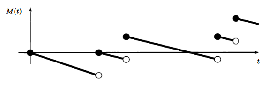
The most fundamental pure jump process is the Poisson process, which is flat almost everywhere, except for what the process makes a jump which is of size 1. Poisson processes are covered under the stochastic processes sections. One property to keep in mind is that Poisson processes are cadlag.
Extensions of the Poisson process
Let $N(t)$ be a Poisson process. In order to make it a martingale, the monotonic increasing $N(t)$ should be demeaned. Of course at a given $N(t)$, $\E(N(t)) = \lambda t$ so one should expect $N(t)-\lambda t$ to be a martingale wrt the canonical filtration. This is the compensated Poisson process which looks like
The reader should check that this is indeed a martingale.
Another form of a Poisson process is a compound Poisson process. It is a process in which the jumps are of random height, defined by the following.
\[Q(t) = \sum_{i=1}^{N(t)}Y_i\]Here $N(t)$ is a Poisson process and $Y_i$’s are iid random variables with mean $\beta$ independent of $N(t)$. $Y_i$ is not restricted to positive values, so jumps can be negative. Its expectation is:
\[\E(Q(t)) = \E\left(\E\left(\sum_{i=1}^{N(t)} Y_i \vert N(t)\right)\right) = \E(N(t)\E(Y_i|N(t))) = \E(N(t)\E(Y_i)) = \E(N(t))\E(Y_i) = \lambda \beta t\]Therefore, $Q(t) - \beta\lambda t$ should be expected to be a martingale. (Reader should check that this is true).
The compound Poisson process $Q(t)$ has independent increments, and stationary increments like the regular Poisson process, as the reader should check.
Decomposition of the Compound Poisson Process
Suppose we have $y_1,..,y_m$ non-zero numbers such that $\sum_{i=1}^m p(y_i) = 1$. Suppose we also have the Poisson processes $N_1(t),…,N_m(t)$ each with mean $\lambda p(y_i)$. We define the following:
\[Q(t) = \sum_{i=1}^M y_i N_i(t)\]Here $Q(t)$ is a compound Poisson process. To see this:
- Note that the superposition of $N_1,…,N_m$ poisson processes yield another Poisson process with rate $\lambda$.
- $Q(t)$ in the above, can be written as a sum $\sum_{i=1}^{N(t)} y_i$
And as a corrolary, for a given compound Poisson process $Q(t) = \sum_{i=1}^{N(t)} Y_i$, and jumps of size $y_k$ for $k=1,…,m$, we can let $N_k(t)$ be the number of jumps of size $y_k$. Then we can rewrite $Q(t)$ as:
\[Q(t) = \sum_{i=1}^m y_i N_i(t)\]which uses Poisson thinning to reduce $N(t) = \sum_{i=1}^m N_i(t)$.
Jump Processes
The reason why we want to define jump processes are due to the following integral:
\[\int_0^T \Delta(t) dX(t)\]where $X(t)$ is a process that has jumps. Perhaps $\Delta(t)$ can be a process denoting the holdings of a particular asset and $X(t)$ the price of the asset. Then the integral tracks the total value of the holding up to time $T$.
We define a jump process as a process that can be represented as the sum of an Ito integral, Riemann integral, and a pure jump process. It is right continuous, due to the jump process, so the continuous portion of the process is soley due to the Ito and Riemann portions.
\[X(T) = X_0 + \int_0^T \Gamma(s)dW(s) + \int_0^T \Theta(s)ds + J(t)\]Since $J(t)$ is required to be a pure jump process, $J(t)$ can either be a compound Poisson, or a Poisson process, if restricting our jump processes to the examples above.
The continuous version of the jump process is:
\[X^C(T) = X_0 + \int_0^T \Gamma(s)dW(s) + \int_0^T \Theta(s)ds\]Integral of Jump Processes
The integral of a jump process is defined as follows. Suppose we want to integrate some adapted process $\Phi(t)$ wrt a jump process $X(t)$, i.e. $\int_0^T \Phi(t)dX(t)$. We define the integral as:
\[\int_0^T \Phi(t)dX(t) = \int_0^T \Phi(t)\Gamma(t)dW(t) + \int_0^T \Phi(t)\Theta(t)dt + \sum_{0<t<T}\Phi(t)\Delta J(t)\]We define $\Delta J(t)$ as $J(t)- J(t-)$ which is the jump size for the points in $t$ where $J$ is right continuous. This captures the jump size of the jump process.
Quadratic Variation
The QV of the jump process defined on the continuous portion is $\int_0^T \Gamma^2(s)ds$. The sketch is as follows:
- Discretize the partitions and treat the integrals as left sums as in the Ito sense
- Show cross term is 0, by using the same strategy as in the Ito processes case
- Show the cross terms in the $(\sum)^2$ terms are all 0
- Show that the sum of $\theta^2(t_k)(t_{k+1}-t_k)^2$ is 0
- Show that the sum of $\Gamma^2(t_k)(W(t_{k+1})-W_{t_k})^2 \to \int_0^T \Gamma^2(s)ds$ which was done in the Ito Processes section.
First we discretize the partitions in the Ito sense,
\[\begin{align*} [X^C(t_{j+1})-X^C(t_{j})]^2 &= \left(\sum_{k=0}^{n-1} \Gamma(t_k)(W(t_{k+1})-W(t_k)) + \sum_{k=0}^{n-1} \Theta(t_k)(t_{k+1}-t_k)\right)^2 \\ &= \left(\sum_{k=0}^{n-1} \Gamma(t_k)(W(t_{k+1})-W(t_k)) + \sum_{k=0}^{n-1} \Theta(t_k)(t_{k+1}-t_k)\right)^2\\ &= \left(\sum_{k=0}^{n-1} \Gamma(t_k)(W(t_{k+1})-W(t_k))\right)^2 + \left(\sum_{k=0}^{n-1} \Theta(t_k)(t_{k+1}-t_k)\right)^2 + \\ &\qquad \qquad 2 \left(\sum_{k=0}^{n-1} \Gamma(t_k)(W(t_{k+1})-W(t_k))\right)\left(\sum_{k=0}^{n-1} \Theta(t_k)(t_{k+1}-t_k)\right) \end{align*}\]The cross-term is shown to be 0 in the same manner as done in the past. Bound the sum by $\max(W(t_{k+1})-W(t_k)) \times \max(t_{k+1} - t_k)$, which converge to 0 as partition sizes shrink. Likewise, the sum involving $\Theta(t_k)$ can also be zeroed in a similar manner. In the exact same manner as done in the Ito-Doeblin thereom under Ito Processes, we can deduce that
\[\left(\sum_{k=0}^{n-1} \Gamma(t_k)(W(t_{k+1})-W(t_k))\right)^2 \stackrel{n\to\infty}{\to} \int_0^T \Gamma^2(s)ds\]which can be heuristically deduced using Box calculus, described in the Ito process section.
In the jump process $X_1(t)$ and $X_2(t)$, we can also consider the cross variation which is defined as
\[\lim_{n\to\infty} \sum_{j=0}^{n-1} (X_1(t_{j+1})-X_1(t_j))(X_2(t_{j+1})-X_2(t_j))\]We demonstrate that \(Q_{X_1}(T) = \int_0^T \Gamma_1^2(s)ds + \sum_{0 < t < T}\Delta J_1(t)\)
\[C_{X_1,X_2}(T) = \int_0^T \Gamma_1(s)\Gamma_2(s) ds + \sum_{0 < t < T}\Delta J_1(t)\Delta J_2(t)\]The sketch is as follows:
- We only show the $C_{X_1,X_2}(T)$ result, as $Q_{X_1}$ is a special result of $C_{X_1,X_2}(T)$.
- Break up $X_1$ and $X_2$ into $X_1^C, X_2^C, J_1, J_2$
- Recall that $C_{X_1^C, X_2^C}(T) = \int_0^T \Gamma_1(t)\Gamma_2(t)dt$
- Show that $C_{J_1,J_2}(T) = \sum_{0<t<T}\Delta J_1(t)\Delta J_2(t)$.
- Show that $C_{X_k,J_k}(T) = 0$
From Box calculus, step 5 should be clear since $J$ does not involve any Ito integral terms, while $X$ does. Any terms that do not involve Ito integrals, will have a cross variation of 0.
\[\begin{align*} \sum_{j=0}^{n-1} (X_1(t_{j+1})-X_1(t_j))(X_2(t_{j+1})-X_2(t_j)) &= \sum_{j=0}^{n-1} (X_1^C(t_{j+1})-X_1^C(t_j) + J_1(t_{j+1}) - J_1(t_j)) \times \\ &\qquad (X_2^C(t_{j+1})-X_2^C(t_j) + J_2(t_{j+1}) -J_2(t_j)) \\ &= \sum_{j=0}^{n-1} (X_1^C(t_{j+1})-X_1^C(t_j))(X_2^C(t_{j+1})-X_2^C(t_j)) + \\ &\qquad \sum_{j=0}^{n-1} (X_1^C(t_{j+1})-X_1^C(t_j))(J_2(t_{j+1}) -J_2(t_j)) + \\ &\qquad \sum_{j=0}^{n-1} (X_2^C(t_{j+1})-X_2^C(t_j))(J_1(t_{j+1}) -J_1(t_j)) + \\ &\qquad \sum_{j=0}^{n-1} (J_1(t_{j+1}) -J_1(t_j))(J_2(t_{j+1}) -J_2(t_j)) \end{align*}\]By continuity of $X^C$, the second and third terms are 0. The argument is the same for both terms. The key is that $\sum \Delta J_i < \infty$ in finite time.
\[\begin{align*} &\sum_{j=0}^{n-1} (X_1^C(t_{j+1})-X_1^C(t_j))(J_2(t_{j+1}) -J_2(t_j)) \\ &\leq \max\{(X_1^C(t_{j+1})-X_1^C(t_j))\}\sum_{j=0}^{n-1}(J_2(t_{j+1}) -J_2(t_j)) \\ &\to 0 \end{align*}\]Finally,
\[\sum_{j=0}^{n-1} (J_1(t_{j+1}) -J_1(t_j))(J_2(t_{j+1}) -J_2(t_j)) = \sum_{0<t<T} \Delta J_1(t) \Delta J_2(t)\]Stochastic Calculus for Jump Processes
The jump process has a continuous portion and a jump portion, where the continuous portion is identical to the diffusion Ito process. So if $X(t)$ is a jump diffusion process, then $X^C(t)$ follows:
\[\partial f(t, X^C(t)) = f_x(t, X^C(0))\Gamma(t)\partial W(t) + f_t(X^C(t))\Theta(t)dt + \frac{1}{2}f_{xx}(t, X^C(t))\Gamma^2(t)dt\]Now we add the jump term $J(t)$ into the process to get the jump diffusion process. Jumps are finite on the interval, so for times $t$ where there is no jump, the Ito lemma above holds.
If there is a jump, we must incorporate the jump height, which is given by $\Delta J(t_i) = J(t_i) - J(t_i -)$. This is the same as $X(t_i)-X(t_i-)$ so
\[\begin{align*} f(T, X(T)) &= f(0, X(0)) + \int_0^T f_x(t, X^C(0))\Gamma(t)d W(t) + \int_0^T f_t(t, X^C(t))\Theta(t)dt + \\ &\qquad \frac{1}{2}\int_0^T f_{xx}(t, X^C(t))\Gamma^2(t)dt + \sum_{0<t<T} (f(t, X(t)) - f(t, X(t-))) \end{align*}\]This forms the Ito-Doeblin lemma for jump diffusion processes with one jump process.